Section One

Project Overview

The following page is a deployment/visualization of clustering and classification project results based on the web. This project aims to fulfill the final assignment of the Dicoding course by meeting six criteria, which include:

The clustering project started with loading the data then followed by Exploratory Data Analysis (include missing value, duplicated data and outliers identification), data preprocessing (include data cleaning and data encoding, standardization & normalization), Clustering Model Development (include feature selection with grid search, model selection and model evaluation) and Cluster Visualization. The final evaluation of the model indicated a good performance, achieving a silhouette score about 59%. The data labeled with the cluster was then exported to a CSV file. The file is then used for the classification project.

The classification project began with loading the file then followed by data splitting (7:3), Classification Model Development (with Random Forest), Hyperparameter Tuning with grid search, and Model Evaluation. It turns out that the model's performance was poor, with very low accuracy and F1 score. Undersampling and Oversampling was used to handle the problem. The last evaluation of the model showed that the model's performance was good, with accuracy and F1 score above 90%.

As explained earlier, this page only presents the results and its visualizations of the clustering and classification project. For more details, you can access it through the following link: Machine Learing for Clustering, Machine Learing for Classification

Section Two

The Dataset

Customer Personality Analysis Dataset

---

Customer Personality Analysis is an in-depth analysis of the ideal customers for a company. It helps businesses better understand their customers and enables them to tailor products according to the specific needs, behaviors, and interests of different customer types.

Customer personality analysis allows businesses to adjust their products based on the target customers from various segments. For example, instead of spending money marketing a new product to all customers in the company's database, the company can analyze which customer segments are most likely to purchase the product and then market it only to that segment.

This dataset was chosen from the "Suggested Dataset Sources" in the Machine Learning Project Submission.

Number of rows: 2240 | Number of columns: 29 | Dataset Source: Dataset Link (Kaggle)

Section Three

Clustering

Modeling without Feature Selection

---

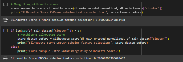
In this project, two models were selected, namely DBSCAN and K-Means, to be tested without prior feature selection. The evaluation results using silhouette score were 0.590 (K-Means) and 0.22 (DBSCAN).

The K-Means model shows good performance, but the issue is that it uses too many features, which can make interpreting the clustering results more difficult. It means the features selection was needed.

Modeling with Feature Selection

---

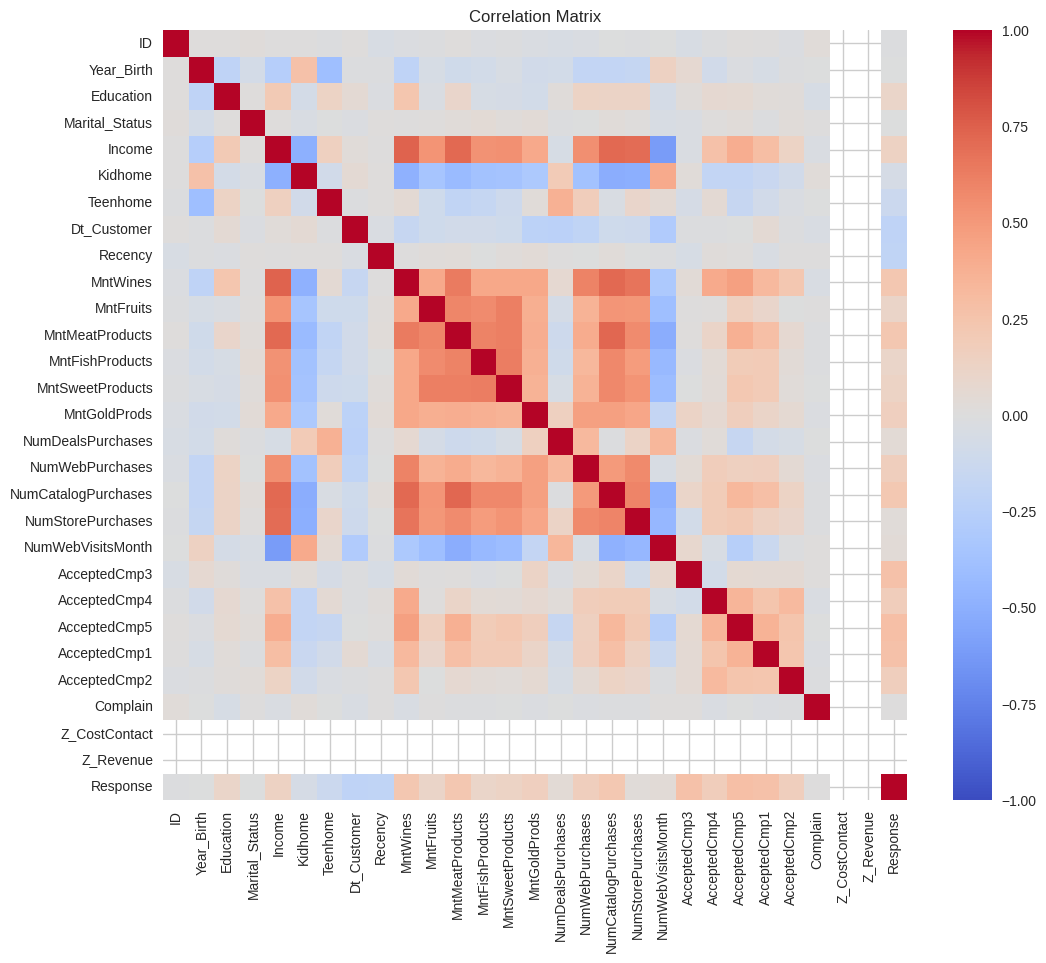
To solve the issue, Correlation Matrix was used to show which features has the most significant correlation to each other.

Based on the correlation matrix, 16 features are considered, with 5 or 6 to be selected for model training. Here are the 16 features:

Since we select 5 or 6 out of 16, It will take so much times if we select them manually.

Mathematically, if we selected 5 out of 16 features, we will need C_16^5=16!/(16-5)!5!=4368 trial to find the best 5 features (globally optimal) and C_16^6=16!/(16-6)!6!=8008 trial for the best 6 features selection. From here, the grid search was used to find the best 5 or 6 features, since 8008 trial was considered as ‘not a really big number’ to do the grid search.

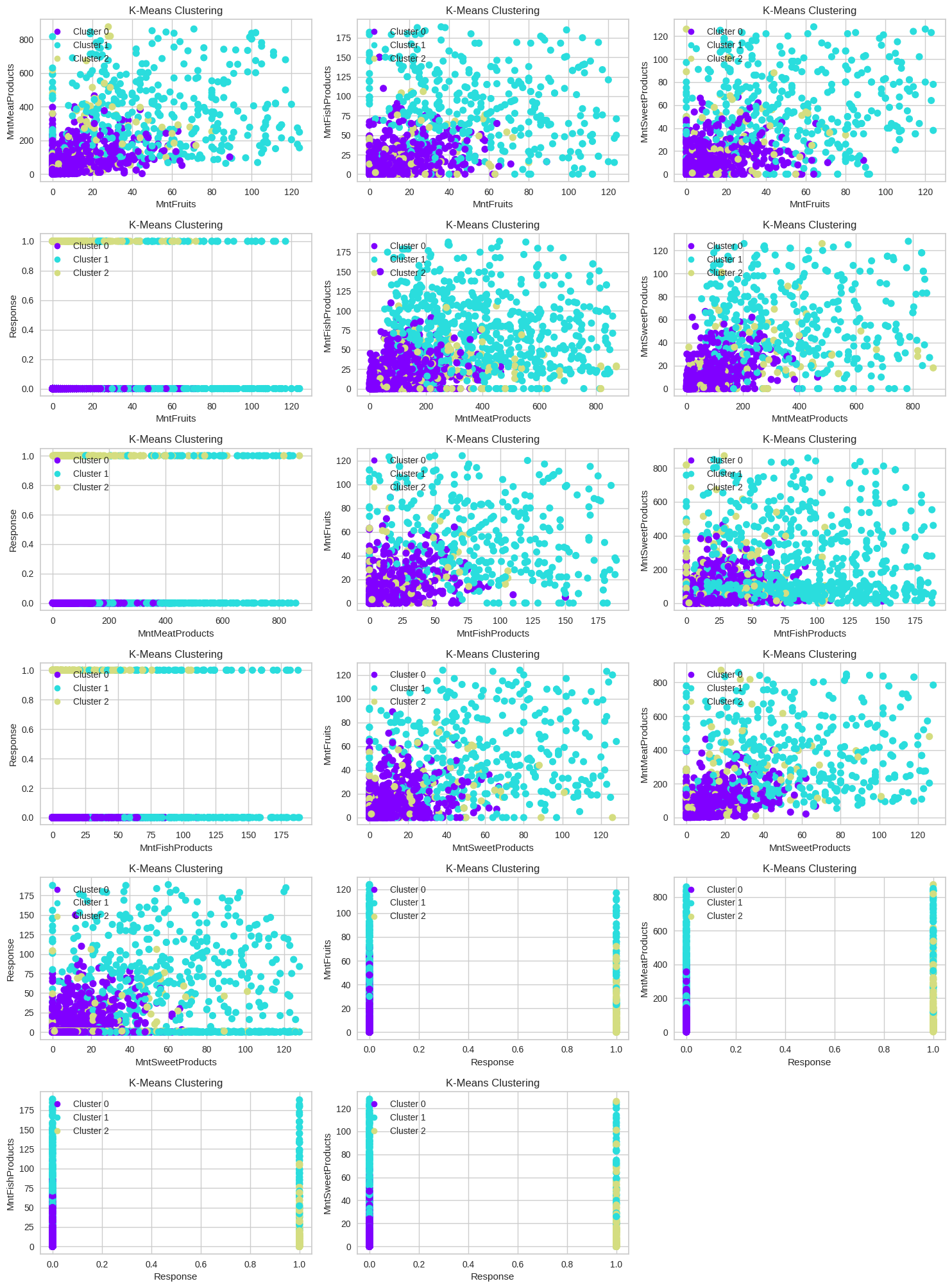
The grid search applied to K-Means clustering showed that the best 5 features were MntFruits, MntMeatProducts, MntFishProducts, MntSweetProducts, and Response, with a total of 3 clusters and a 0.593 silhouette score. This was better than the first K-Means model, where feature selection was not applied, because the second model had less features and better Silhouette Score.

In contrast, the best 6 features, MntFruits, MntMeatProducts, MntFishProducts, MntSweetProducts, MntGoldProds, and Response, produced 5 clusters with a silhouette score of 0.522, which doesn’t meet the minimum silhouette score requirements and was worse than the model with the best 5 features. It means

DBSCAN was not used in this case due to the extensive time required for feature selection and hyperparameter tuning. Since the DBSCAN and K-Means models with the best 6 features were not used, the only remaining option is the K-Means model with the best 5 features.

Cluster Visualization

---

The K-Means with best 5 features was visualized with matplotlib. Here is the visualization:

Cluster Interpretation

---

Here is the conclusion of the cluster interpretation. To see more detailed process of this part, visit the google colab link: Machine Learing for Clustering

Section Four

Classification

Modeling without Hyperparameter Tuning

---

The labeled data with cluster numbers was exported for use in the ML-Classification project. The model used in this project is the Random Forest Classifier. Initially, the data was split into a 70:30 ratio. The 70% portion was then used to train the model with default hyperparameters. The model's performance is as follows:

Modeling with Hyperparameter Tuning

---

The model appears to exhibit overfitting, as it performs well on the training data but significantly worse on the testing data. To address this issue, Hyperparameter Tuning was conducted. Grid Search was chosen as the Hyperparameter Tuning algorithm for this project. The following parameter grid was considered:

After completing hyperparameter tuning, the best model was selected and its performance evaluated. Below is a comparison of the model's performance before and after hyperparameter tuning:

Modeling after Oversampling and Undersampling

---

The model after hyperparameter tuning appears to exhibit underfitting, as indicated by poor performance on both the training and testing data. To address this issue, Oversampling and Undersampling methods were applied. Once these methods were implemented, the model was trained both with and without hyperparameter tuning. Below is a comparison of the model's performance before and after hyperparameter tuning.